Parameter-space ReSTIR for Differentiable and Inverse Rendering

SIGGRAPH North America 2023 (Conference Track)

Table of Contents

Description

Physically-based inverse rendering algorithms that utilize differentiable rendering typically use gradient descent to optimize for scene parameters such as materials and lighting. We observe that the scene often changes slowly from frame to frame during optimization, similar to animation, and therefore adapt temporal reuse from ReSTIR to reuse samples across gradient iterations and accelerate inverse rendering.

Presentation

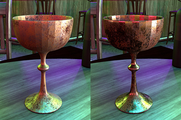
Result: Optimizing the Roughness Texture of a Tire

We optimize a 2048x2048 roughness texture of the tire in a scene with multiple colored lights. By reusing samples from previous iterations, our method converges faster than the Mitsuba 3 baseline, as shown by the glossy highlights.

Key Insights

1. Optimization as Animation

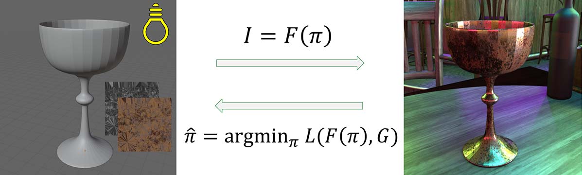
In inverse rendering, we aim to recover scene parameters such as materials and lighting from a target image or photo. We can optimize for this iteratively using gradient descent by:

1. Rendering an image $\image$ using the parameters $\params$.
2. Comparing the rendered image $\image$ with the target image $\refimage$ using a loss function $\loss(\image,\refimage)$.
3. Updating the parameters with the derivative of the loss with respect to each parameter: $\params^{(i+1)} = \params^{(i)} - \boldsymbol\alpha^{(i)} \ppd{\loss}{\params^{(i)}}$.
4. Repeating 1-3 until convergence.

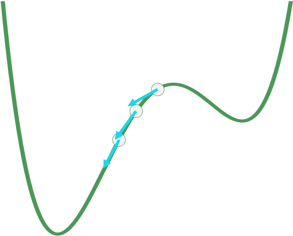
We observe that at every iteration, the scene only changes by a single (often small) gradient step. As a result, during optimization, the scene changes slowly, and the sequence of frames we render often looks like an animation. This observation inspires us to apply algorithms designed for animation and real-time rendering, and in this paper, we apply the ReSTIR algorithm in particular to reuse samples across gradient descent iterations.

2. Parameter-centric Algorithms for Differentiable Rendering

Forward rendering algorithms typically compute a single quantity – the pixel color – for each pixel in the image. We call these image-centric algorithms, since the focus is on pixels in the image. On the other hand, the goal of differentiable rendering is to compute derivatives. In inverse rendering, these are the derivatives of the loss function with respect to the parameters. For example, if we wish to optimize a texture describing the color of an object, then these derivatives are $\ppd{\loss}{\param_1}, \ppd{\loss}{\param_2}, \cdots, \ppd{\loss}{\param_n}$ for texels $\param_1, \param_2, \cdots, \param_n$.

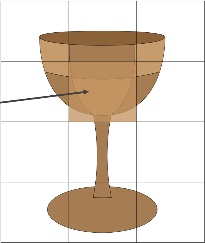
However, most differentiable rendering algorithms are still image-centric! They compute each above derivative for every pixel, and sum across all pixels to compute the final derivatives. For example, to compute the derivative at texel 1, we would sum over all pixels $j$ to compute $$ \ppd{\loss}{\param_1} = \sum_j \ppd{\loss(I_j, G_j)}{\param_1}. $$ In our paper, we show that we can reformulate differentiable rendering to be parameter-centric: that is, we can directly compute a single value per parameter, instead of computing values at each individual pixel. We show that for a parameter $\pi_i$, this is: $$ \ppd{\loss}{\param_i} = \int_\Omega \ppw(\ex) \ppd{}{\param_i} f_c(\ex, \params) \diff\mu(\ex). $$ Intuitively, $\ppd{}{\param_i} f_c(\ex, \params)$ describes how changing the parameter $\pi_i$ affects the light carried by light path $\ex$, and $\ppw(\ex)$ describes how this change affects the loss function defined across the entire image. We claim that this can be the more natural formulation for differentiable rendering, and is particularly crucial for applying ReSTIR, which needs to store a reservoir for each derivative. See the paper for further details.

3. Resampled Importance Sampling for Real-valued Functions

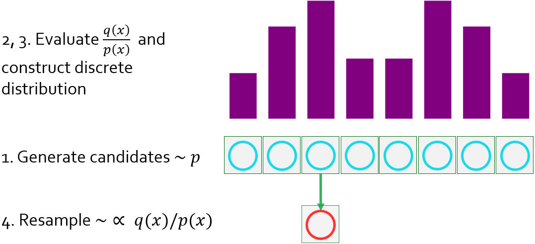
Resampled importance sampling (RIS) is a method to approximately importance sample an arbitrary target function $q$, which is otherwise intractable to sample from directly. It accomplishes this by:

1. Drawing $M$ candidate samples $x_1, x_2, \cdots, x_M$ from a source distribution $p$ that we know how to sample from.
2. Evaluating the weight $w_s = q(x_s) / p(x_s)$ for each candidate $x_s$.
3. Building a discrete probability distribution $P(z) = w_z / \sum_{s=1}^M w_s$.
4. Selecting a sample $x_z$ (resampling) out of the pool of candidates with probability $P(z)$.

As $M$ increases, $x_z$ becomes closer to being distributed according to $q^*$ (the normalized target distribution). In the limit as $M\to\infty$, $x_z$ becomes a sample drawn exactly from $q^*$.

We can then use $x_s, x_z$ to estimate an integral $F = \int f(x) \diff x$ with the estimator $$ \estimator{F} = \frac{f(x_z)}{q(x_z)} \frac{1}{M} \sum_{s=1}^M \frac{q(x_s)}{p(x_s)}. $$ In concrete terms, as an example, in the original ReSTIR paper, RIS is used to sample direct lighting, where $f$ is the integrand of the rendering equation, $q \approx f$ (lighting and BRDF, without visibility), and $p$ is the density of light sampling.

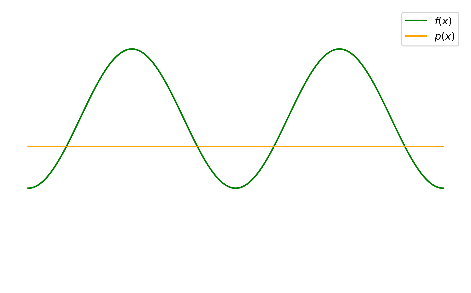
An issue that arises when applying RIS to differentiable rendering, is that unlike in forward rendering, our integrand $f$, which is a derivative, is now real-valued, i.e. it can take both positive and negative values. However, since $q$ is an unnormalized target distribution, it has to be non-negative. This means that even if we could perfectly importance sample according to $q=\abs{f}$, we would still have variance due to differences in sign across samples.

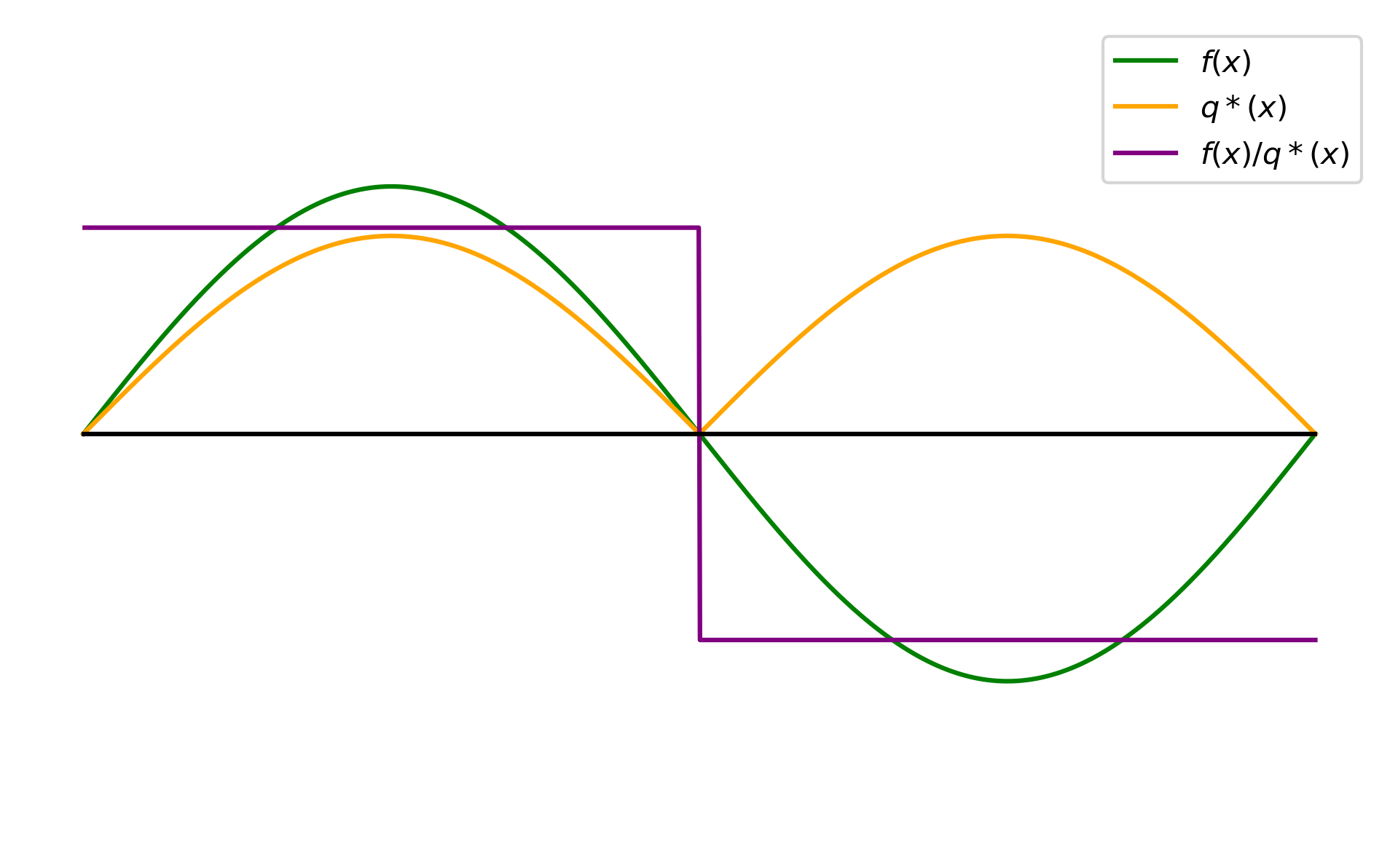
Our solution is to borrow ideas from positivization, which decomposes $f$ into a positive part $f_+$ and a negative part $f_-$, and importance samples them separately. In particular, we split $q$ into $q_+$ and $q_-$: $$ q_+(x) = \max{(q(x), 0)} \qquad q_-(x) = \max{(-q(x), 0)} \ $$ and use the estimator: $$ \estimator{F} = \frac{f(x_{z+})}{q_+(x_{z+})} \frac{1}{M} \sum_{s=1}^M \frac{q_+(x_s)}{p(x_s)} + \frac{f(x_{z-})}{q_-(x_{z-})} \frac{1}{M} \sum_{s=1}^M \frac{q_-(x_s)}{p(x_s)} $$ In simpler terms, all this means is that we draw samples from $p$ as usual, evaluate $q(x_s)$, and categorize them into positive and negative samples based on the sign of $q(x_s)$. The positive samples then effectively estimate the region of $q$ that is positive, and the negative samples estimate the region of $q$ that is negative. Then, if $q=f$, our estimator does achieve zero-variance in the limit. In practice, we apply this strategy to generalized RIS, a method we call Positivized GRIS or PGRIS.

BibTeX

@inproceedings{Chang2023ReSTIRDiffRender,
  title = {Parameter-space ReSTIR for Differentiable and Inverse Rendering},
  author = {Chang, Wesley and Sivaram, Venkataram and Nowrouzezahrai, Derek and
  Hachisuka, Toshiya and Ramamoorthi, Ravi and Li, Tzu-Mao},
  booktitle = {ACM SIGGRAPH 2023 Conference Proceedings},
  articleno = {18},
  numpages = {10},
  year = {2023},
  publisher = {Association for Computing Machinery},
  address = {New York, NY, USA},
  location = {Los Angeles, CA, USA},
  series = {SIGGRAPH '23},
  url = {https://doi.org/10.1145/3588432.3591512},
  doi = {10.1145/3588432.3591512}
}